Pitot tube flow meter
The working principle of pitot tubes for measurement of volumetric flow
 30 May 2020
In this post, we will take a closer look at the pitot tube flow meter. We will discuss the different pitot tube types and look for the underlying principles that ensure that the pitot tube does what it should do, that is to measure the flow velocity.
But let’s start from the beginning.
What is a pitot tube?
A pitot tube, named after the French engineer Henri Pitot, is the sensing element of a differential pressure measurement that is used to measure the flow velocity of liquids and gases, including steam.
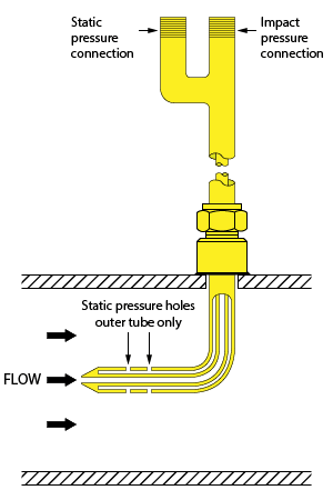
Classical designs have an L-shaped double-walled tube with the open end facing upstream and eventually one or more holes in the outer tube wall behind the open end. The inner and outer tube walls are connected to each other at the front hole, while at the other end both tubes are available for connection to a differential pressure instrument.
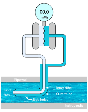
More recent designs are made of a straight multi-chamber tube, perpendicular to the flow direction, with multiple holes in the front and the rear chamber of the tube. Both chambers come out separately at the top of the pitot tube for connection to the pressure instrument.
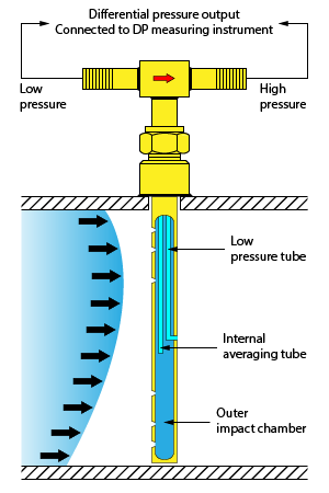
The DP signal from the pitot tube can be measured by a differential pressure transmitter which then converts the signal to a flow velocity provided that the density of the fluid is known. By combining a pitot tube and a differential pressure transmitter, we get a pitot tube flow meter.
When the pitot tube is installed in a conduit with a known cross-sectional area, it becomes possible to calculate the volumetric flow by multiplying the measured flow velocity by the cross-sectional area.
Further multiplication of the volume flow by the density of the fluid gives us the mass flow rate.
The pitot tube flow meter working principle
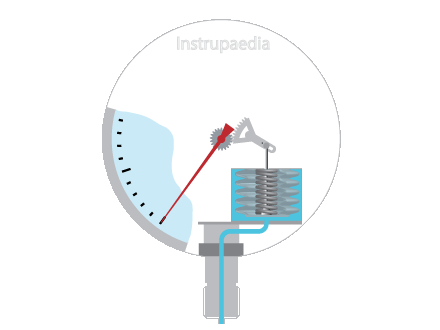
The drawing above is showing a classical pitot tube inserted into a conduit with the tube opening oriented against the flow.
If the fluid is not flowing, the pressure will be the same in the inner and outer tubes. This pressure is called static pressure.
As soon as the fluid starts to flow, a part of the fluid will enter the pitot tube through its front hole, but it has nowhere to go because the inner tube is closed at the back as it is connected to the pressure transmitter. So, once the tube has filled up, the fluid will come to a standstill (stagnation) inside the tube.
However, the fluid continues to flow through the conduit and the molecules build up kinetic energy. Because the fluid can no longer enter the pitot inner tube, all molecules will collide at the front hole. This brings them to a full stop and they lose their kinetic energy.
But energy is never lost. So, with every collision, the kinetic energy is converted into pressure energy.
The pressure built up at the tip of the pitot tube is called the stagnation pressure, sometimes also called the total pressure. It is the sum of the static pressure, equally distributed in all directions, and the dynamic pressure, caused by the conversion of the kinetic energy and effective in the flow direction only.
Stagnation pressure = static pressure + dynamic pressure
A number of small holes were drilled in the outer tube. Since these openings are perpendicular to the direction of flow, they are not influenced by the dynamic pressure. They are only subjected to static pressure.
We could say that the inner tube is sensing the stagnation pressure, while the outer tube is sensing the static pressure.
A pitot tube that measures both the stagnation and the static pressure is called a pitot-static tube or Prandtl tube. If the two tubes coming out of the pitot-static tube are connected to a differential pressure transmitter, as shown in de animation above, we can measure the dynamic pressure of the fluid flow.
Dynamic pressure = ΔP = Pstagnation – Pstatic
We will need the result of this measurement to calculate the flow velocity of the fluid.
To find the formula for the calculation of the flow velocity, we have to start from the basic principle, the Bernoulli equation:
P1 + 1 2 ρV12 = P2 + 1 2 ρV22
Those who are not familiar with this formula should read the article about the Bernoulli principle first, as that will explain how we arrive at this formula.
In the above equation, the potential energy terms (ρgh) have already been canceled because we are assuming a horizontal flow.
The velocity V2 at the front hole of the pitot tube is stagnated. This means that V2 is equal to zero, and we can delete the full term 1 2 ρV22.
This simplifies the equation to:
P2 – P1 = ΔP = 1 2 ρV12
Solving for V1 gives us the flow velocity in the conduit:
V1 = √ 2ΔP ρ
| Where: | V1 | = | velocity of the fluid |
| ΔP | = | the measurement value of the pressure transmitter | |
| ρ | = | density of the fluid |
With the velocity of the fluid now known, we can obtain the volumetric flow rate by multiplying the velocity by the cross-sectional area of the conduit.
Qv = A1V1 = Π 4 D2 √ 2ΔP ρ
| Where: | Qv | = | volumetric flow rate |
| A1 | = | cross-sectional area | |
| D | = | diameter of the conduit |
Even the mass flow rate can now be calculated if we multiply the volumetric flow rate by the density of the fluid.
Qm = ρQv = ρ Π 4 D2 √ 2ΔP ρ
| Where: | Qm | = | mass flow rate |
Or, if you don’t want a fraction under the square root:
Qm = Π 4 D2√ 2ΔPρ
The density of the fluid can be obtained as follows:
- When the pressure and the temperature of the fluid are constant, the density can be found in a density table for that specific fluid. That value can then be programmed into the control system.
- When the temperature and the pressure change continuously, these need to be measured and their measured value sent to the control system. The density table for that specific fluid must then be programmed into the control system so that the system can select the density value that corresponds to the pressure and temperature it has received.
It has to be said that to arrive at these formulas, we had to make the following assumptions:
- The fluid we are measuring is incompressible
- There are no dissipative forces (heat loss, friction)
- The fluid is non-viscous
- The flow is steady laminar
Different types of pitot tubes
L-type pitot tube
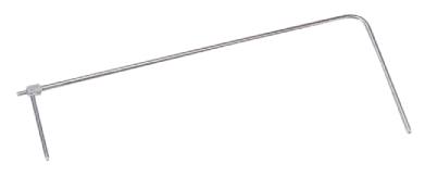
This is a basic pitot-static tube like the one I used for the animation above. It has the typical L-shape consisting of the head, which has to be aligned with the fluid flow, and the stem which passes through the wall of a conduit. The length of the head is generally between 15 and 25 times the head diameter.
The tip of the head has a front hole that is connected to a smaller tube that runs inside the head and stem and comes out the other side parallel to the stem. This inner tube transfers the total pressure registered by the front hole.
The tip of the L-type pitot tube can be designed in 3 different ways:
- a spherical shaped tip (AMCA type)
- an ellipsoidal shaped tip (NPL type)
- a conical shaped tip (CETIAT type)

Eight static pressure holes are drilled around the circumference of the head at a distance of 6 to 8 times the head diameter from the tip. The static pressure is transferred through the outer tube and comes out at a branch perpendicular to the stem. This branch also serves as an alignment arm to facilitate head alignment since the visibility of the head is obstructed by the conduit wall.
A standard pitot tube provides acceptable gas velocity measurements as long as the tube direction does not deviate more than 15° from the flow direction. When the deviation exceeds 15°, the dynamic pressure reading decreases rapidly.
S-type pitot tube
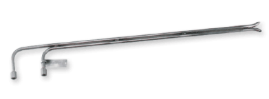
The probe is inserted into the conduit with its total pressure hole upstream, facing the flow, and its static pressure hole downstream pointing in the direction of the flow. The faces of both openings must be perpendicular to the flow.
The large openings of typically 4 – 10 mm permit the S-type probe to be used in gases containing dust or fine droplets. The large holes are not easily plugged and therefore these types of pitot tubes are often used for flow measurement in emission stacks.
Because the total pressure hole is obstructing the flow to the static pressure hole and given the size of these holes, the flow profile at the static pressure hole will be disturbed.
As a result :
- The measured static pressure will be lower than the real static pressure. To compensate for this difference, the S-type pitot tube must be calibrated.
- The measured differential pressure will be higher compared to the L-type pitot tube, which is beneficial in low-velocity gas flow applications.
Just like the L-type pitot tube, the S-pitot tube provides an acceptable measurement when the direction of the gas flow does not deviate more than 15° from the direction of the pitot tube.
Rotating the S-tube by 90°, so it stands perpendicular to the flow direction, leads to a measured differential pressure that equals zero.
This makes it possible to determine the flow direction of the gas and the tangential flow angle, by rotating the S-pitot tube until the measured differential pressure is zero.
The tangential flow angle is the angle between the flow direction of the gas and the axial direction of the conduit.
If the tangential flow angle is greater than 15°, then the velocity corrected for flow direction is given by:
vc = cosθmeasvmeas
| Where: | vc | = | velocity corrected for flow direction |
| cosθmeas | = | cosine of the tangential flow angle | |
| vmeas | = | velocity measured at angle θmeas |
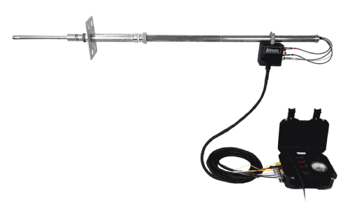
3D pitot tube
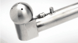

This type of probe consists of 5 pressure taps in a spherical (or prism-shaped) sensor head. The pressure taps are numbered P1 to P5 in a fixed sequence.
Inside the pitot probe are five separate tubes connecting each pressure tap with the measuring device for evaluation of the measured pressure.
The temperature of the gas is measured by a thermocouple on the stem of the probe.
A 3D-probe is used in a particular case when stack gas has a flow profile with a significant yaw angle and pitch angle. In this case, the L- or S-probes would lose too much of their accuracy to perform a reliable measurement.
The 3D-probe can determine the yaw and pitch angle and the dynamic pressure by using its 5 pressure taps.
- To find the yaw angle the probe is rotated around its axis until the differential pressure P2 – P3 equals zero. This operation is called yaw nulling. An inclinometer will then calculate the yaw angle and its value will be displayed on the console.
- The differential pressure P4 – P5 is used to calculate the pitch angle using probe-specific calibration curves.
- The differential pressure P1 – P2 is a function of total velocity.
From these values and a determination of the gas density, the average axial velocity of the gas is calculated.
The average gas volumetric flow rate can be found by multiplying the average axial velocity by the cross-sectional area of the conduit.
2D pitot tube

The 2D probe may look the same as the 3D probe (both can be prism-shaped) but has only 3 pressure taps, numbered P1, P2, and P3, at the same spot as the 3D probe.
Therefore, the 2D probe can only measure the velocity pressure and the yaw angle.
- P1 – P2 determines the velocity pressure
- P2 – P3 is used to find the yaw angle
From these measurements and the density of the gas, the average near-axial velocity of the gas is calculated.
Notice that a 2D probe only measures the near-axial velocity, since it ignores the pitch component of the flow.
Multiplying the near-axial velocity by the cross-sectional area of the pipe gives the average gas volumetric flow rate.
It is also possible to use a 3D as a 2D probe by operating the 3D probe in the yaw determination mode only.
Related topics
1 Comment
Leave a Comment
Your email address will not be published. Fields marked with * are required.


Your style is really unique in comparison to other people I have read stuff from. I appreciate you for posting when you’ve got the opportunity, Guess I’ll just bookmark this blog.